Create a plot for a neural network model

The function uses the plotnet function of the NeuralNetTools R package to draw a neural network plot and visualize the hidden layer structure.

Usage

nplot(object, hidden, bias = TRUE, sleep = 2, ...)

Arguments

object: A neural network model object
hidden: The hidden structure of the object
bias: A logical value, indicating whether to draw biases in the layers (default = FALSE).
sleep: Suspend plot display for a specified time (in secs, default = 2).
...: Currently ignored.

Value

The function invisibly returns the graphical objects representing the neural network architecture designed by NeuralNetTools.

Details

The induced subgraph of the input graph mapped on data variables. Based on the estimated connection weights, if the connection weight W > 0, the connection is activated and it is highlighted in red; if W < 0, the connection is inhibited and it is highlighted in blue.

References

Beck, M.W. 2018. NeuralNetTools: Visualization and Analysis Tools for Neural Networks. Journal of Statistical Software. 85(11):1-20.

Author

Mario Grassi mario.grassi@unipv.it

Examples


# \donttest{
if (torch::torch_is_installed()){

# load ALS data
ig<- alsData$graph
data<- alsData$exprs
data<- transformData(data)$data

#ncores<- parallel::detectCores(logical = FALSE)
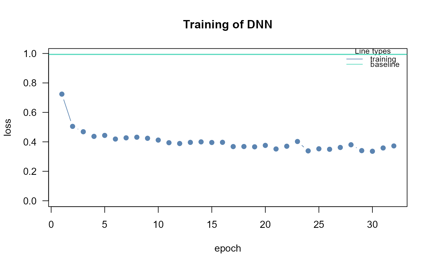
dnn0 <- SEMdnn(ig, data, train=1:nrow(data), algo = "layerwise",
      hidden = c(10, 10, 10), link = "selu", bias =TRUE,
      epochs = 32, patience = 10, verbose = TRUE)

 #Visualize the neural networks per each layer of dnn0
 nplot(dnn0, hidden = c(10, 10, 10), bias = FALSE)
}
#> Conducting the nonparanormal transformation via shrunkun ECDF...done.
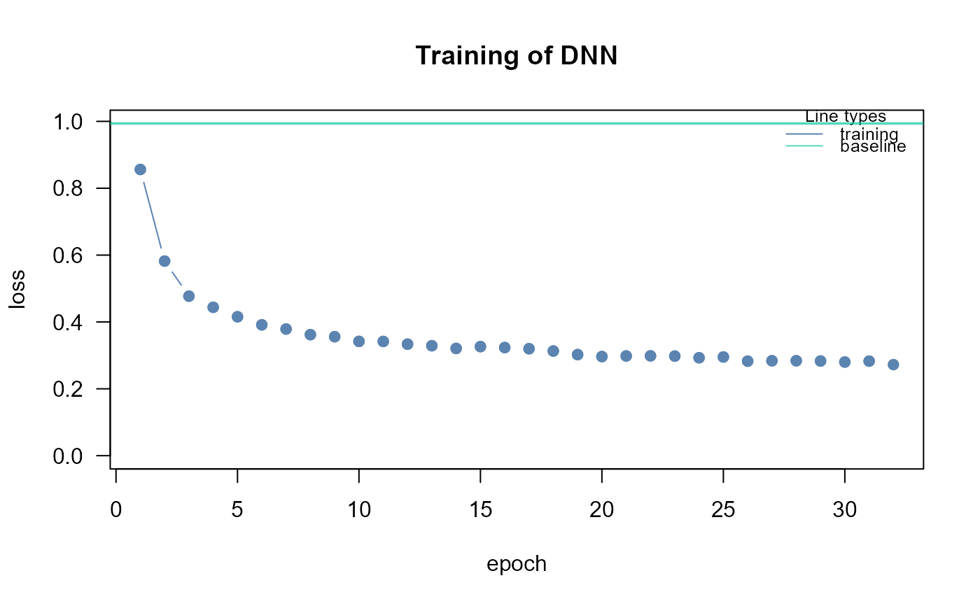
#> Running SEM model via DNN...
#> 
#> layer 1 : z10452 z84134 z836 z4747 z4741 z4744 z79139 z5530 z5532 z5533 ...
#>    train      val     base 
#> 0.445215      Inf 0.993750 
#> 
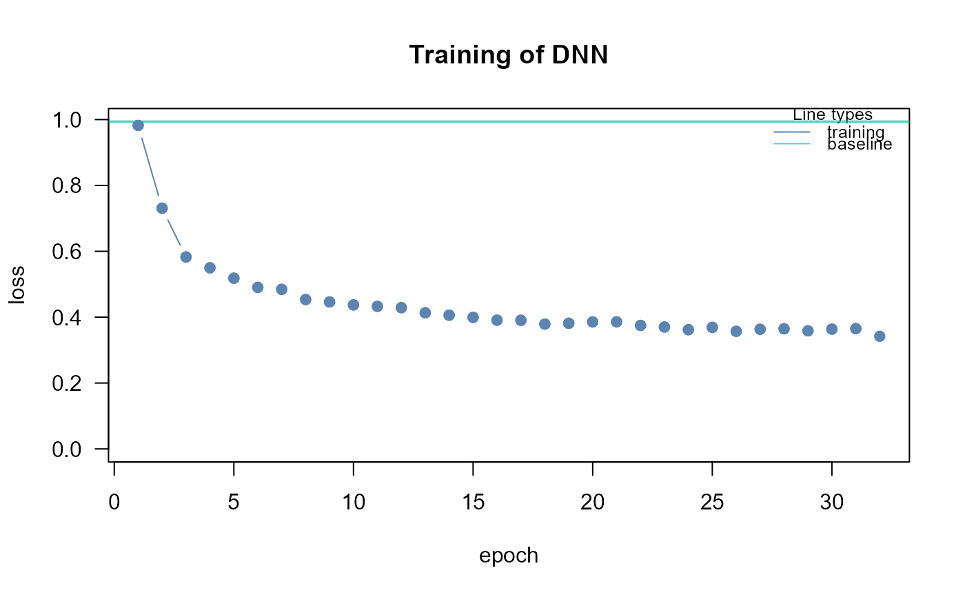
#> layer 2 : z842 z1432 z5600 z5603 z6300 
#>     train       val      base 
#> 0.5153647       Inf 0.9937500 
#> 
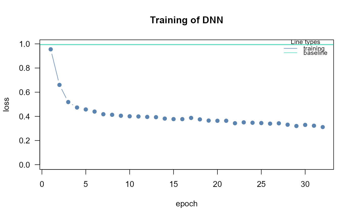
#> layer 3 : z54205 z5606 z5608 
#>     train       val      base 
#> 0.5990095       Inf 0.9937500 
#> 
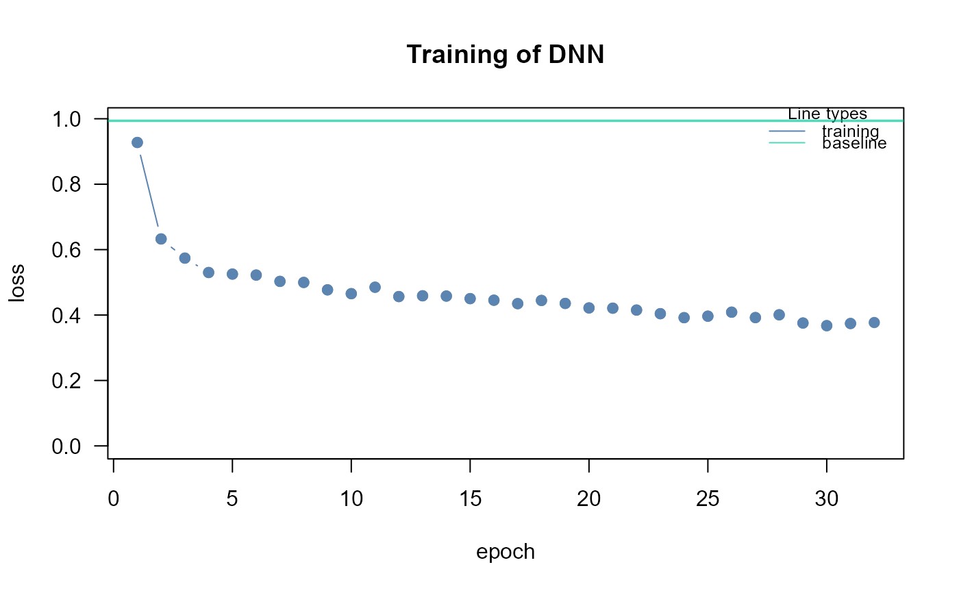
#> layer 4 : z596 z4217 
#>     train       val      base 
#> 0.9540080       Inf 0.9937501 
#> 
#> layer 5 : z1616 
#>     train       val      base 
#> 0.8792974       Inf 0.9937500 
#>  done.
#> 
#> DNN solver ended normally after 160 iterations
#> 
#>  logL:-50.309658  srmr:0.207363





# }