This function computes a model-agnostic variable importance based on a Shapley-value decomposition of the model R-Squared (R2, i.e., the coefficient of determination) that allocates the proportion of model- explained variability in the data to each model feature (Redell, 2019).
Usage
getShapleyR2(
  object,
  newdata,
  newoutcome = NULL,
  thr = NULL,
  ncores = 2,
  verbose = FALSE,
  ...
)
Arguments
- object
A model fitting object from
SEMml(), orSEMrun()functions.- newdata
A matrix containing new data with rows corresponding to subjects, and columns to variables.
- newoutcome
A new character vector (as.factor) of labels for a categorical output (target)(default = NULL).
- thr
A numeric value [0-1] indicating the threshold to apply to the signed Shapley R2 to color the graph. If thr = NULL (default), the threshold is set to thr = 0.5*max(abs(signed Shapley R2 values)).
- ncores
number of cpu cores (default = 2)
- verbose
A logical value. If FALSE (default), the processed graph will not be plotted to screen.
- ...
Currently ignored.
Value
A list od four object: (i) shapx: the list of individual Shapley values of predictors variables per each response variable; (ii) est: a data.frame including the connections together with their signed Shapley R-squred values; (iii) gest: if the outcome vector is given, a data.frame of signed Shapley R-squred values per outcome levels; and (iv) dag: DAG with colored edges/nodes. If abs(sign_r2) > thr and sign_r2 < 0, the edge is inhibited and it is highlighted in blue; otherwise, if abs(sign_r2) > thr and sign_r2 > 0, the edge is activated and it is highlighted in red. If the outcome vector is given, nodes with absolute connection weights summed over the outcome levels, i.e. sum(abs(sign_r2[outcome levels])) > thr, will be highlighted in pink.
Details
Shapley values (Shapley, 1953; Lundberg & Lee, 2017) apply the fair
distribution of payoffs principles from game theory to measure the additive
contribution of individual predictors in a ML model. The function compute
a signed Shapley R2 metric, that combines the additive property of Shapley
values with the robustness of the R-squared (R2) of Gelman (2018) to produce
a variance decomposition that accurately captures the contribution
of each variable in the ML model, see Redell (2019). The signed values are
used in order to denote the regulation of connections in line with a linear
model, since the edges in the DAG indicate node regulation (activation, if
positive; inhibition, if negative). The sign has been recovered for each edge
using sign(beta), i.e., the sign of the coefficient estimates from a linear
model (lm) fitting of the output node on the input nodes (see Joseph, 2019).
Furthermore, to determine the local significance of node regulation in the DAG,
the Shapley decomposition of the R-squared values for each outcome node (r=1,...,R)
can be done by summing the Shapley R2 indices of their input nodes.
It should be noted that the operations required to compute Shapley values processed
with the kernelshap function of the kernelshap R
package are inherently time-consuming, with the computational time increasing in
proportion to the number of predictor variables and the number of observations.
References
Shapley, L. (1953) A Value for n-Person Games. In: Kuhn, H. and Tucker, A., Eds., Contributions to the Theory of Games II, Princeton University Press, Princeton, 307-317.
Scott M. Lundberg, Su-In Lee. (2017). A unified approach to interpreting model predictions. In Proceedings of the 31st International Conference on Neural Information Processing Systems (NIPS'17). Curran Associates Inc., Red Hook, NY, USA, 4768–4777.
Redell, N. (2019). Shapley Decomposition of R-Squared in Machine Learning Models. arXiv preprint: https://doi.org/10.48550/arXiv.1908.09718
Gelman, A., Goodrich, B., Gabry, J., & Vehtari, A. (2019). R-squared for Bayesian Regression Models. The American Statistician, 73(3), 307–309.
Joseph, A. Parametric inference with universal function approximators (2019). Bank of England working papers 784, Bank of England, revised 22 Jul 2020.
Author
Mario Grassi mario.grassi@unipv.it
Examples
# \donttest{
# load ALS data
ig<- alsData$graph
data<- alsData$exprs
data<- transformData(data)$data
#> Conducting the nonparanormal transformation via shrunkun ECDF...done.
#...with train-test (0.5-0.5) samples
set.seed(123)
train<- sample(1:nrow(data), 0.5*nrow(data))
rf0<- SEMml(ig, data[train, ], algo="rf")
#> Running SEM model via ML...
#> done.
#>
#> RF solver ended normally after 23 iterations
#>
#> logL:-33.16687 srmr:0.086188
res<- getShapleyR2(rf0, data[-train, ], thr=NULL, verbose=TRUE)
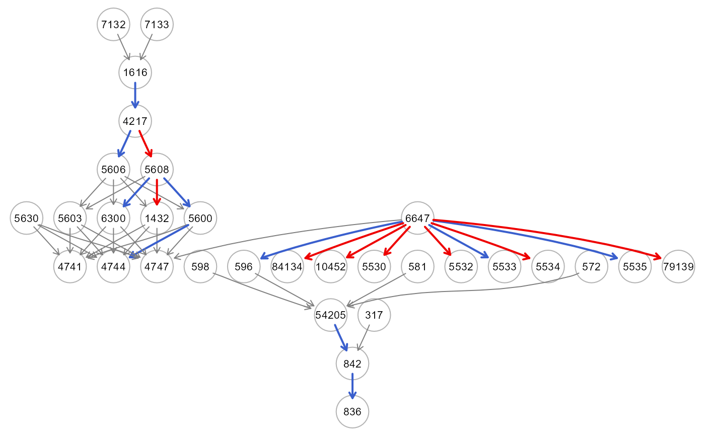 table(E(res$dag)$color)
#>
#> gray50 red2 royalblue3
#> 32 7 6
# shapley R2 per response variables
R2<- abs(res$est[,4])
Y<- res$est[,1]
R2Y<- aggregate(R2~Y,data=data.frame(R2,Y),FUN="sum");R2Y
#> Y R2
#> 1 10452 0.3074106
#> 2 1432 0.2746912
#> 3 1616 0.1025127
#> 4 4217 0.2416770
#> 5 4741 0.2133041
#> 6 4744 0.2336151
#> 7 4747 0.3015739
#> 8 54205 0.2243528
#> 9 5530 0.4424930
#> 10 5532 0.3852137
#> 11 5533 0.3368840
#> 12 5534 0.4944426
#> 13 5535 0.5919868
#> 14 5600 0.2887038
#> 15 5603 0.0000000
#> 16 5606 0.2963567
#> 17 5608 0.5054904
#> 18 596 0.2057984
#> 19 6300 0.3769140
#> 20 79139 0.4867639
#> 21 836 0.5841519
#> 22 84134 0.4718743
#> 23 842 0.3401094
r2<- mean(R2Y$R2);r2
#> [1] 0.3350574
# }
table(E(res$dag)$color)
#>
#> gray50 red2 royalblue3
#> 32 7 6
# shapley R2 per response variables
R2<- abs(res$est[,4])
Y<- res$est[,1]
R2Y<- aggregate(R2~Y,data=data.frame(R2,Y),FUN="sum");R2Y
#> Y R2
#> 1 10452 0.3074106
#> 2 1432 0.2746912
#> 3 1616 0.1025127
#> 4 4217 0.2416770
#> 5 4741 0.2133041
#> 6 4744 0.2336151
#> 7 4747 0.3015739
#> 8 54205 0.2243528
#> 9 5530 0.4424930
#> 10 5532 0.3852137
#> 11 5533 0.3368840
#> 12 5534 0.4944426
#> 13 5535 0.5919868
#> 14 5600 0.2887038
#> 15 5603 0.0000000
#> 16 5606 0.2963567
#> 17 5608 0.5054904
#> 18 596 0.2057984
#> 19 6300 0.3769140
#> 20 79139 0.4867639
#> 21 836 0.5841519
#> 22 84134 0.4718743
#> 23 842 0.3401094
r2<- mean(R2Y$R2);r2
#> [1] 0.3350574
# }