Gradient Weight method for neural network variable importance

The function computes the gradient matrix, i.e., the average marginal effect of the input variables w.r.t the neural network model, as discussed by Scholbeck et al (2024).

Usage

getGradientWeight(object, thr = NULL, verbose = FALSE, ...)

Arguments

object: A neural network object from SEMdnn() function.
thr: A numeric value [0-1] indicating the threshold to apply to the gradient weights to color the graph. If thr = NULL (default), the threshold is set to thr = 0.5*max(abs(gradient weights)).
verbose: A logical value. If FALSE (default), the processed graph will not be plotted to screen.
...: Currently ignored.

Value

A list of three object: (i) est: a data.frame including the connections together with their gradient weights, (ii) gest: if the outcome vector is given, a data.frame of gradient weights for outcome lavels, and (iii) dag: DAG with colored edges/nodes. If abs(grad) > thr and grad < 0, the edge is inhibited and it is highlighted in blue; otherwise, if abs(grad) > thr and grad > 0, the edge is activated and it is highlighted in red. If the outcome vector is given, nodes with absolute connection weights summed over the outcome levels, i.e. sum(abs(grad[outcome levels])) > thr, will be highlighted in pink.

Details

The gradient weights method approximate the derivative (the gradient) of each output variable (y) with respect to each input variable (x) evaluated at each observation (i=1,...,n) of the training data. The contribution of each input is evaluated in terms of both magnitude taking into account not only the connection weights and activation functions, but also the values of each observation of the input variables. Once the gradients for each variable and observation, a summary gradient is calculated by averaging over the observation units. Finally, the average weights are entered into a matrix, W(pxp) and the element-wise product with the binary (1,0) adjacency matrix, A(pxp) of the input DAG, W*A maps the weights on the DAG edges. Note that the operations required to approsimate partial derivatives are time consuming compared to other methods such as Olden's (connection weight). The computational time increases with the size of the neural network or the size of the data.

References

Scholbeck, C.A., Casalicchio, G., Molnar, C. et al. Marginal effects for non-linear prediction functions. Data Min Knowl Disc 38, 2997–3042 (2024). https://doi.org/10.1007/s10618-023-00993-x

Author

Mario Grassi mario.grassi@unipv.it

Examples


# \donttest{
if (torch::torch_is_installed()){

# Load Sachs data (pkc)
ig<- sachs$graph
data<- sachs$pkc
data<- log(data)

#...with train-test (0.5-0.5) samples
set.seed(123)
train<- sample(1:nrow(data), 0.5*nrow(data))
#ncores<- parallel::detectCores(logical = FALSE)

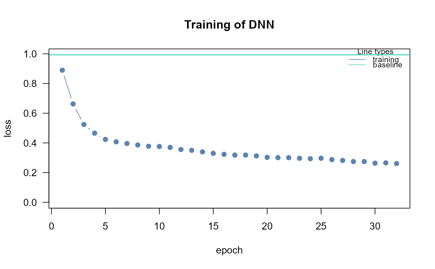
dnn0<- SEMdnn(ig, data[train, ], outcome = NULL, algo= "neuralgraph",
      hidden = c(10,10,10), link = "selu", bias = TRUE,
      epochs = 32, patience = 10, verbose = TRUE)

gw<- getGradientWeight(dnn0, thr = 0.3, verbose = FALSE)
gplot(gw$dag, l="circo")
table(E(gw$dag)$color)
}
#> DAG conversion : TRUE
#> Running SEM model via DNN...
#> Loss at epoch 10: 0.237081, l1: 0.19671
#> Loss at epoch 20: 0.139642, l1: 0.13101
#> Loss at epoch 30: 0.088302, l1: 0.09489
#>  done.
#> 
#> DNN solver ended normally after 32 iterations
#> 
#>  logL:-19.646363  srmr:0.06331

#> 
#>     gray50       red2 royalblue3 
#>         14          3          1 
# }